This page gives an introduction to time-difference-of-arrrival (TDOA) based localization of transmitters and presents a simple practical system using three RTL-SDRs to localize signals in a city. I have presented the work at the Software Defined Radio Academy 2017 in Friedrichshafen, Germany. Because of the great feedback, I decided to put the related material online. The resources can be found at the end of this page.
For further questions please contact me at dc9st<at>panoradio-sdr.de. Furthermore, I would like to say thanks to my former colleague Claus and the Amateur Radio Research Group of TU Kaiserslautern for their support.
Presentation at the Software Defined Radio Academy 2017, Friedrichshafen, Germany
Presentation Slides Download: “Introduction and Experiments on Transmitter Localization with TDOA”
Introduction
Transmitter localization is a both interesting and challenging task. Besides applying triangulation in combination with some type of direction finding receivers (using e.g. directional antennas, pseudo Doppler or the interferometer principle), the Time-Difference-of-Arrival (TDOA) method is widely used. In TDOA three or more (non-directional) receivers at different locations capture the unknown transmitted signal. Then it evaluates the differences in arrival time of the signals to calculate the transmitter’s position (multilateration).
This article first provides a short introduction to localization with TDOA. Second, it presents a simple experimental localization system based on three receivers, each consisting of a RTL-SDR USB-Stick and a Raspberry PI. Although the receivers and the overall setup are very simple, localization of transmitters works remarkably well.
Basics of TDOA
Assume a signal is emitted by an (unknown) transmitter and is received by several receivers at different locations. Usually the signal arrives at different times at the different receivers due to the varying distances between transmitter and receivers. This difference in arrival time is called “TDOA”. A TDOA value can be measured between a pair of receivers. It should be emphasized, that we work on the time difference of arrival, since any absolute arrival times in relation to transmission times are in general not available (as opposed to other localization techniques like time-of-arrival, TOA).
To understand the idea of TDOA localization, consider a simple example based on only two receivers and an unknown transmitter as depicted in the figure below. First, assume that the signal arrives at both receivers at the same point in time, i.e. TDOA = 0s. Then it is obvious, that the distance from the transmitter to receiver 1 is the same as to receiver 2. The transmitter must be located somewhere on a straight line in the middle between the two receivers. This is not yet a unique position, but narrows the possible positions to a line.
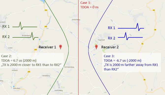
Now assume a second case, where the signal arrives earlier at receiver 1 and later at receiver 2. The TDOA value now becomes non-zero. This means, that the distance from transmitter to receiver 1 is smaller as to receiver 2 (Note, that a TDOA value can be converted to a distance by multiplication with propagation speed). In this case, the possible locations lie on a hyperbola with one of the receivers in its focal point.
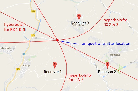
To complete localization, more than two receivers are required – at least three for two dimensional localization in a plane. The above described method to create hyperbolas is applied pairwise to each receiver, such that for three receivers three hyperbolas can be generated (four receivers would yield ten hyperbolas). Ideally, all hyperbolas intersect at a single location on the map, that is the transmitter’s position.
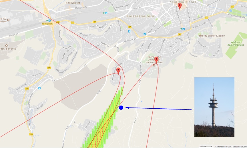
The achievable resolution and accuracy on a map does not only correspond to the resolution of the TDOA measurement. It is also largely dependent of the transmitter’s location relative to the receivers. The resolution figure below shows, that the accuracy is very good in the area roughly between the receivers and poor elsewhere. In general, TDOA systems perform well in the area that is surrounded by the receivers.

Although the basic idea of TDOA localization is not too complicated, some further issues need to be addressed: First, it is required to synchronize the receivers with each other in time. Second, a means of precisely determining the time differences of arrivals must be used. Third, all receivers must be placed apart, though connected and able to exchange considerable amounts of raw sampled data. These challenges need to be solved to build a practical system and will be treated in the following.
A Simple TDOA Localization System using RTL-SDRs
A complete TDOA system consists of three synchronized receivers, that are connected to a central signal processing unit. In the following, a simple and cheap system for localizing signals in a city will be described.
Receivers
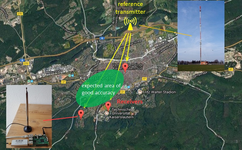
The installed receivers are minimalistic and consist each of a RTL-SDR USB-stick (~20 $) and a Raspberry PI (~40 $). The receivers use the simple whip antenna delivered with the RTL-SDR dongle. For practical reasons the antennas had to be placed indoor, which is suboptimal and leaves room for improvement. The RTL-SDR is capable of receiving 2 MHz of instantaneous bandwidth in a range from below 100 MHz to more than 1 GHz. This makes it a cheap and versatile general purpose SDR, capable of receiving various different types of signals.
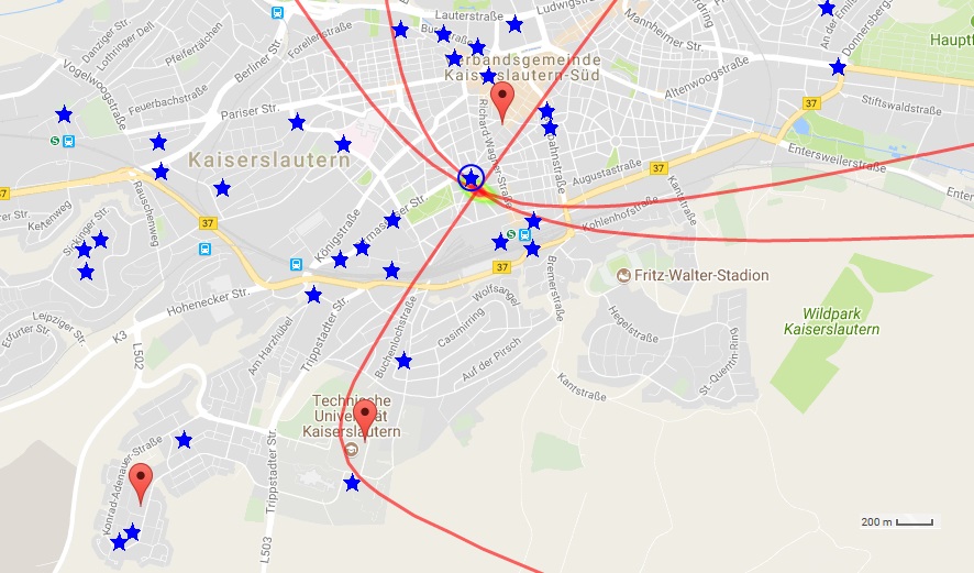
For the experiments three receivers were deployed around in the city of Kaiserslautern, Germany. The figure below shows the receiver’s positions. For ideal placement and good accuracy the receivers should have been placed outside the city. However, in the surrounding, mostly forestal, areas no suitable internet connection could be established. Despite the suboptimal placement, good accuracy is expected in the area roughly between the receivers.
All receivers are connected to a master PC for signal processing via internet. The master triggers measurements at each receiver (simultaneously). Then the receivers send the received sampled data back to master for further signal processing and delay analysis. The amount of sampled data can quickly become very large, since the RTL-SDR outputs 8 bit IQ-data with 2 MHz. This creates a data rate of 2 x 8 bit x 2 MHz = 32 Mbit/s per receiver. With an available DSL upload of 1 Mbit/s, transferring only 1 s of sampled data already takes approximately half a minute. Reducing the sample rate of the RTL-SDR or employing compression may relax data rates.
It is important, that the three receivers are tuned to exactly the same frequency. For that purpose the RTL-SDR’s frequencies are calibrated with special frequency correction busts, emitted by GSM base stations. Calibration with GSM signals is easy using the kalibrate-rtl software.
Synchronization
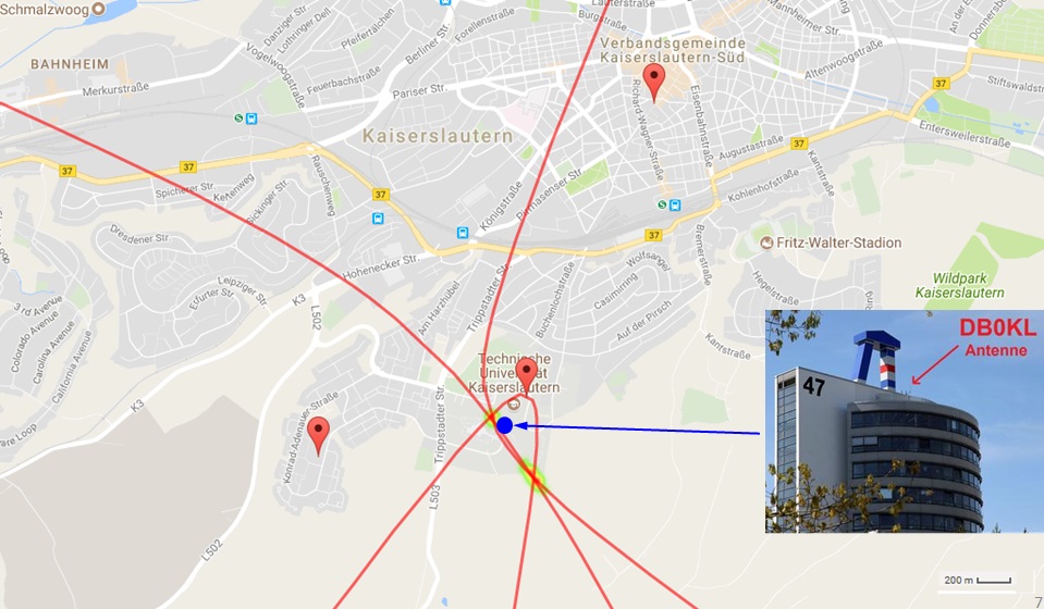
As mentioned above, a prerequisite for TDOA localization is the synchronization of the receivers. One possibility is to use a GPS receiver, that disciplines the Raspberry PI’s internal clock. However, the system utilizes a different method using a transmitter with known location as a reference, that is received well by all three receivers. There is a DAB+ transmitter (217 MHz, 2 kW) in the city of Kaiserslautern, that covers a large area and is perfect for synchronization.
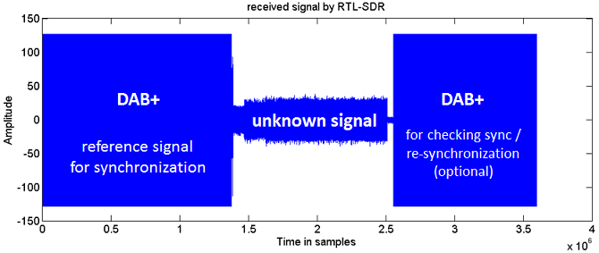
Synchronization with a reference receiver works as follows: When the master triggers a measurement, each receiver first receives some samples of the reference receiver and then seamlessly switches to the unknown transmitter’s signal of interest. For synchronization, the master aligns the three receptions from the different receivers to each other on the time axis. Alignment is done in such a way, that the delay in the reference signal portion corresponds to the known distances of the reference transmitter to the receivers. Once the complete received signal is synchronized (or aligned) the TDOA of the unknown signals is simply calculated as the delay. Precisely spoken, this technique does not synchronize the receivers themselves, but rather the received signals.
The critical point for the synchronization is the requirement to switch between the frequencies seamlessly, such that not a single sample gets lost (otherwise, this will impair synchronization). Modifying the C library librtlsdr (commonly used for controlling the RTL-SDR) to perform seamless frequency switching using the “rtl_sdr” command made it crash during execution. The solution is to use a modified branch of the librtlsdr, called “async-rearrangements” as a basis. Modifying this library for seamless frequency switching worked perfectly fine and showed that the RTL-SDR can do so.
The modified lib librtlsdr-2freq for switching between two frequencies is available as open source software.
Signal Processing for TDOA
Measuring the delay between two inputs precisely is the most important operation for TDOA. For that purpose the correlation function is suitable. It is defined as
Corr(\tau) = \sum_{t=0}^{N-1}s_1(t)s_2(t+\tau)(s1, s2 are the real signals received by RX1 and 2) and outputs for every hypothetical delay \tau between the two signals a value indicating how good the two signals match. The delay value of \tau, at which the correlation function has a peak is the delay between the signals (see also my detailed description of correlation and Steven W. Smith: The Scientist and Engineer’s Guide to Digital Signal Processing, 1997).
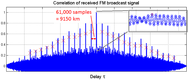
However, in practice several challenges occur. The quality of correlation (desired: a single, unique peak) depends on many factors such as signal bandwidth, periodicity, multi-path propagation, noise, transmitted content and the fact that both signals went through different receivers. The figures below show the correlation functions of real-world signals, captured with two RTL-SDRs placed at different locations. The DAB signal has a very good correlation with a dominant and distinct peak. The correlation function for the FM signal is of poorer quality, showing many outstanding spikes and no distinct peak sample.
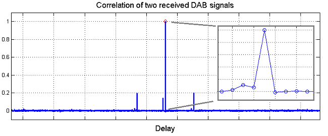
The problem identifying a single sample as correlation peak can be improved by simply smoothing the correlation function with a moving average filter.
The problem of multiple peaks can often be solved by considering the values on the time delay axis of the correlation function. For the FM signal the distance between the peaks is comparably large, around 61,000 samples, which corresponds to a difference in distance of 9150 km. However, the maximum possible delay is the distance between the two receivers (here: a few kilometers). Therefore any peaks that correspond to (positive or negative) delays greater than the receiver’s distance can be discarded. Often, this leaves only a single peak even with correlation functions that look very difficult at first sight.
The correlation function as introduced above assumes real valued data as inputs. The RTL-SDR, however, outputs complex I/Q data. Different experiments were conducted, that used complex correlation, correlation on the absolute values of complex I/Q and the phase difference of complex I/Q data. It turned out that the method using phase differences was mostly suitable for a wide range of different signals. More information on correlation here.
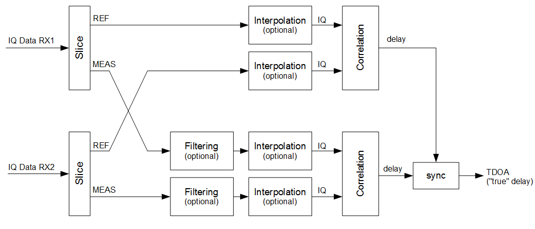
With the correlation function available for measuring the delay or TDOA and having synchronized the receptions, the overall signal processing for TDOA localization can be summarized:
- Receive signals, transfer them to the master and consider them pairwise for further processing
- Synchronize the received signals
- Calculate correlation of reference signal portion
- Discard invalid peaks of correlation function
- Use measured delay to synchronize
- Measure unknown signals
- Calculate correlation of unknown signal portion
- Discard invalid peaks of correlation function
- Determine TDOA in samples and distance
- Calculate hyperbola using geometry
- Create a map with html and javascript (Google maps or Open Street Map) to display the results
The signal processing has been implemented as Matlab/Octave script and is available for download.
Results
The results show the localization of four different transmitters of various signals: a DMR signal at 439 MHz, a mobile phone signal at 922 MHz, a FM signal at 96.9 MHz and an unknown signal at 391 MHz. The results are remarkably good and show that localization is possible even with this simple setup.

Further Development
Since the presented system is very simple, numerous improvements can be made to increase accuracy, reliability and speed:
- Use compression of IQ data or modern methods such as compressed sensing to decrease the amount of data to be transferred and move towards real time processing
- Use a 4th receiver for 3-D localization with height information
- Use a better radio (e.g. higher sampling rate, more stable clocks), better antenna and better placed antenna to improve accuracy
- Include mechanisms to detect failures and intolerable errors, e.g. due to unfavorable signal content
- Set up a “spatial receiver” showing a map (instead of a waterfall), that shows signal sources with transmitting frequency
Resources:
- Raspberry PI images and instructions on how to set up a TDOA system
- https://github.com/DC9ST/librtlsdr-2freq – librtlsdr-2freq, the modified librtlsdr for switching frequencies during reception
- https://github.com/DC9ST/rtl-sdr-data-read – a matlab script for reading data recorded with the “rtl_sdr” command
- https://github.com/DC9ST/tdoa-evaluation-rtlsdr– Matlab/Octave scripts to perform multilateration with TDOA
- Further Comments on the relationship between Signal Properties, Correlation Method and Correlation Quality